Screening visualizations
These visualizations are intended as a way to test the integrity and utility of the data export and cleaning workflow.
Setup
screen_df <- readr::read_csv(file.path(here::here(), "data/csv/screening/agg/PLAY-screening-datab-latest.csv"))## Rows: 641 Columns: 68
## ── Column specification ──────────────────────────────────────────────────
## Delimiter: ","
## chr (54): session_name, session_release, participant_ID, participant_...
## dbl (10): session_id, vol_id, child_age_mos, child_birthage, child_we...
## lgl (1): pilot_pilot
## dttm (1): submit_date
## date (2): session_date, participant_birthdate
##
## ℹ Use `spec()` to retrieve the full column specification for this data.
## ℹ Specify the column types or set `show_col_types = FALSE` to quiet this message.Dates & times
To calculate cumulative screening/recruiting calls by site, we have to add an index variable
Calls across time
df |>
    dplyr::filter(!is.na(submit_date), !is.na(n_calls), !is.na(site_id)) %>%
    ggplot() +
    aes(submit_date, n_calls, color = site_id) +
    geom_point()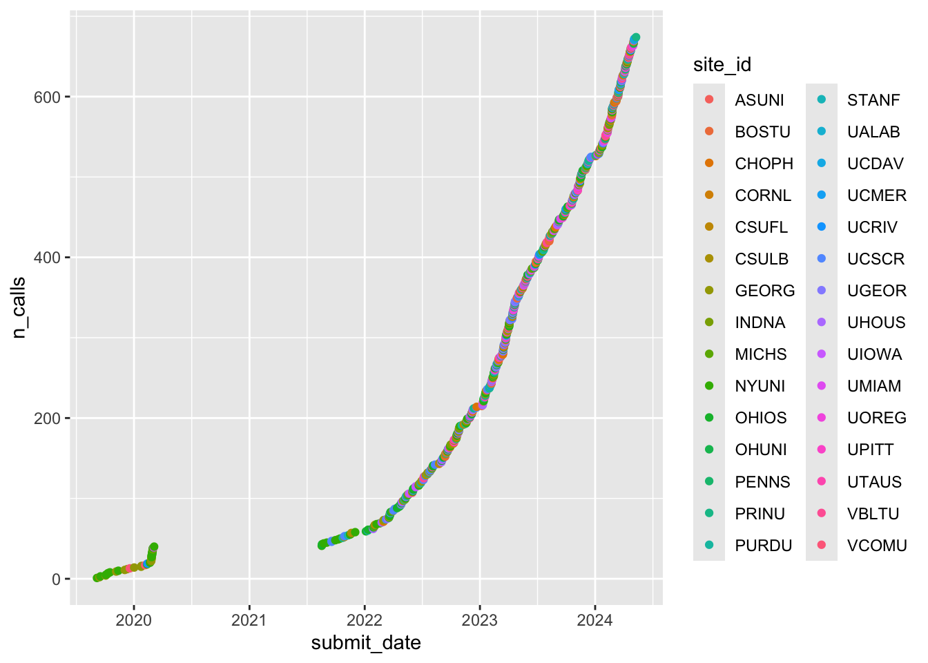
Figure 1: Cumulative screening calls by year and site
Calls by site
calls_by_site_plot <- function(df) {
  df |>
    filter(!is.na(site_id)) %>%
    ggplot() +
    aes(fct_infreq(site_id), fill = site_id) +
    geom_bar() +
    theme(axis.text.x = element_text(
      angle = 90,
      vjust = 0.5,
      hjust = 1
    )) + # Rotate text
    labs(x = "site") +
    theme(legend.position = "none")
}

calls_by_site_plot(df)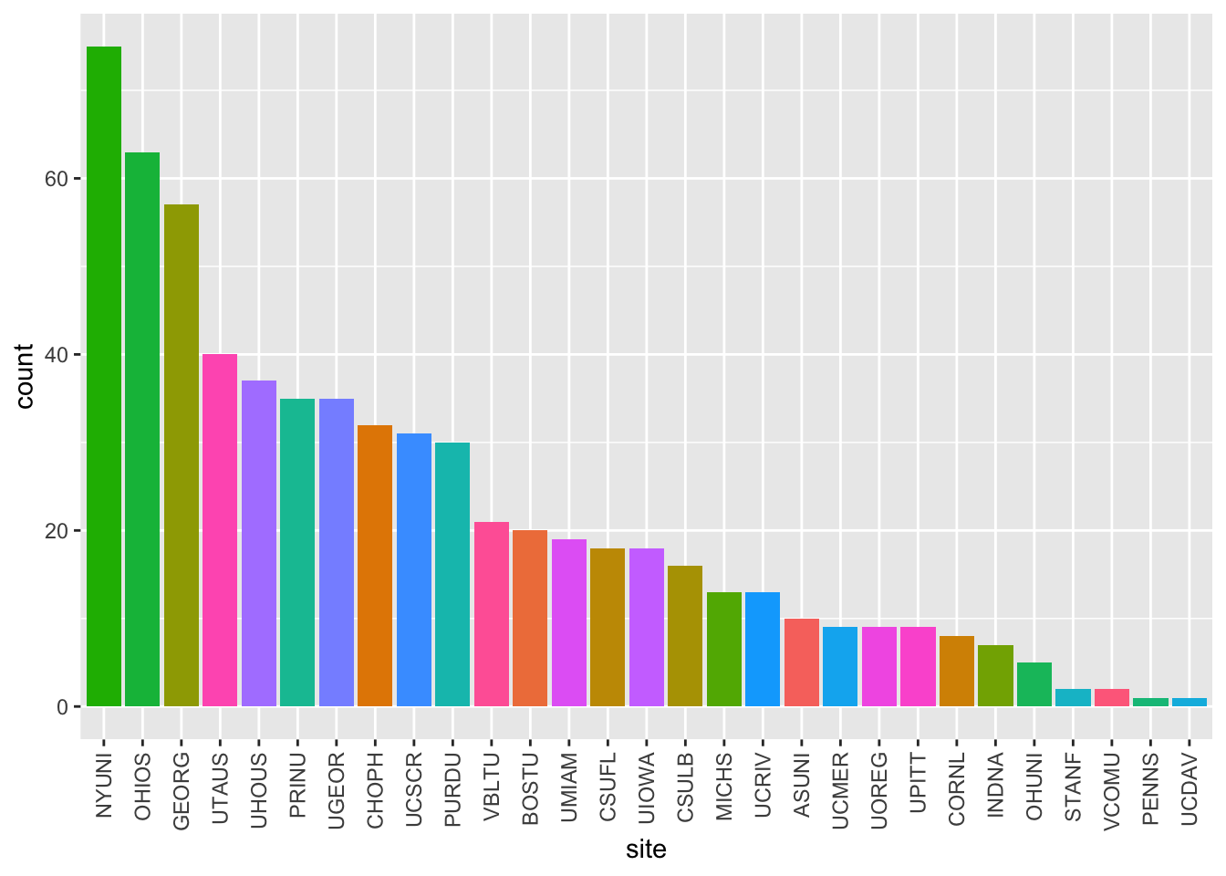
Figure 2: Cumulative screening calls by site
Demographics
Child age
Child age in months (child_age_mos) by child_sex.
screen_df |>
  dplyr::filter(!is.na(child_age_mos), !is.na(child_sex)) |>
  ggplot() +
  aes(child_age_mos, fill = child_sex) +
  geom_histogram(bins = 50)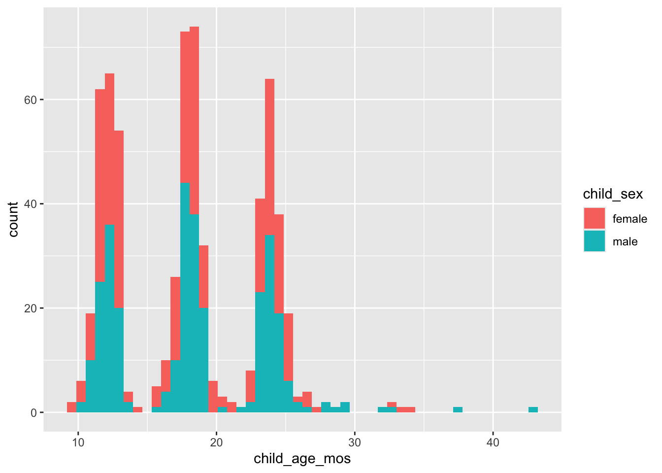
Figure 3: Histogram of child age at time of recruiting call.
Some of the code to clean the screen_df variables could be incorporated into an earlier stage of the workflow.
Language
To child
Language(s) spoken to child by child_sex.
df <- screen_df |>
  dplyr::mutate(
    language_spoken_child = stringr::str_replace_all(language_spoken_child, " ", "_"),
    language_spoken_home = stringr::str_replace_all(language_spoken_home, " ", "_")
  )

xtabs(formula = ~ child_sex + language_spoken_child,
      data = df)
## language_spoken_child
## child_sex english english_other english_spanish english_spanish_other
## female 264 2 44 2
## male 239 4 51 1
## language_spoken_child
## child_sex spanish
## female 13
## male 15At home
xtabs(formula = ~ child_sex + language_spoken_home, data = df)## language_spoken_home
## child_sex english english_other english_spanish english_spanish_other
## female 268 3 34 1
## male 228 3 61 2
## language_spoken_home
## child_sex other spanish
## female 1 14
## male 1 14To child vs. at home
xtabs(formula = ~ language_spoken_child + language_spoken_home, data = df)## language_spoken_home
## language_spoken_child english english_other english_spanish
## english 477 2 17
## english_other 2 4 0
## english_spanish 13 0 69
## english_spanish_other 2 0 1
## spanish 2 0 8
## language_spoken_home
## language_spoken_child english_spanish_other other spanish
## english 2 0 4
## english_other 0 0 0
## english_spanish 1 2 6
## english_spanish_other 0 0 0
## spanish 0 0 18Child health
Child born on due date
xtabs(formula = ~ child_sex + child_bornonduedate,
      data = screen_df)
## child_bornonduedate
## child_sex no yes
## female 8 312
## male 7 302There are \(n=\) 12 NAs.
screen_df |>
  dplyr::filter(is.na(child_bornonduedate)) |>
  dplyr::select(vol_id, participant_ID) |>
knitr::kable(format = 'html')| vol_id | participant_ID |
|---|---|
| 1656 | 001 |
| 1008 | 013 |
| 1008 | 013 |
| 1008 | 013 |
| 1008 | 013 |
| 1576 | 003 |
| 1576 | 006 |
| 1481 | 006 |
| 954 | 001 |
| 1103 | 001 |
| 979 | 026 |
| 996 | 015 |
Child term
xtabs(formula = ~ child_bornonduedate + child_onterm,
      data = screen_df)
## child_onterm
## child_bornonduedate no yes
## no 1 14
## yes 1 499Child weight
Must convert pounds and ounces to decimal pounds.
df <- screen_df %>%
  dplyr::mutate(.,
                birth_weight_lbs = child_weight_pounds + child_weight_ounces/16)

df |>
  dplyr::filter(!is.na(birth_weight_lbs), !is.na(child_sex)) |>
  dplyr::filter(birth_weight_lbs > 0) |>
  ggplot() +
  aes(x = birth_weight_lbs, fill = child_sex) +
  geom_histogram(binwidth = 0.33) +
  theme(legend.position = "bottom") +
  theme(legend.title = element_blank())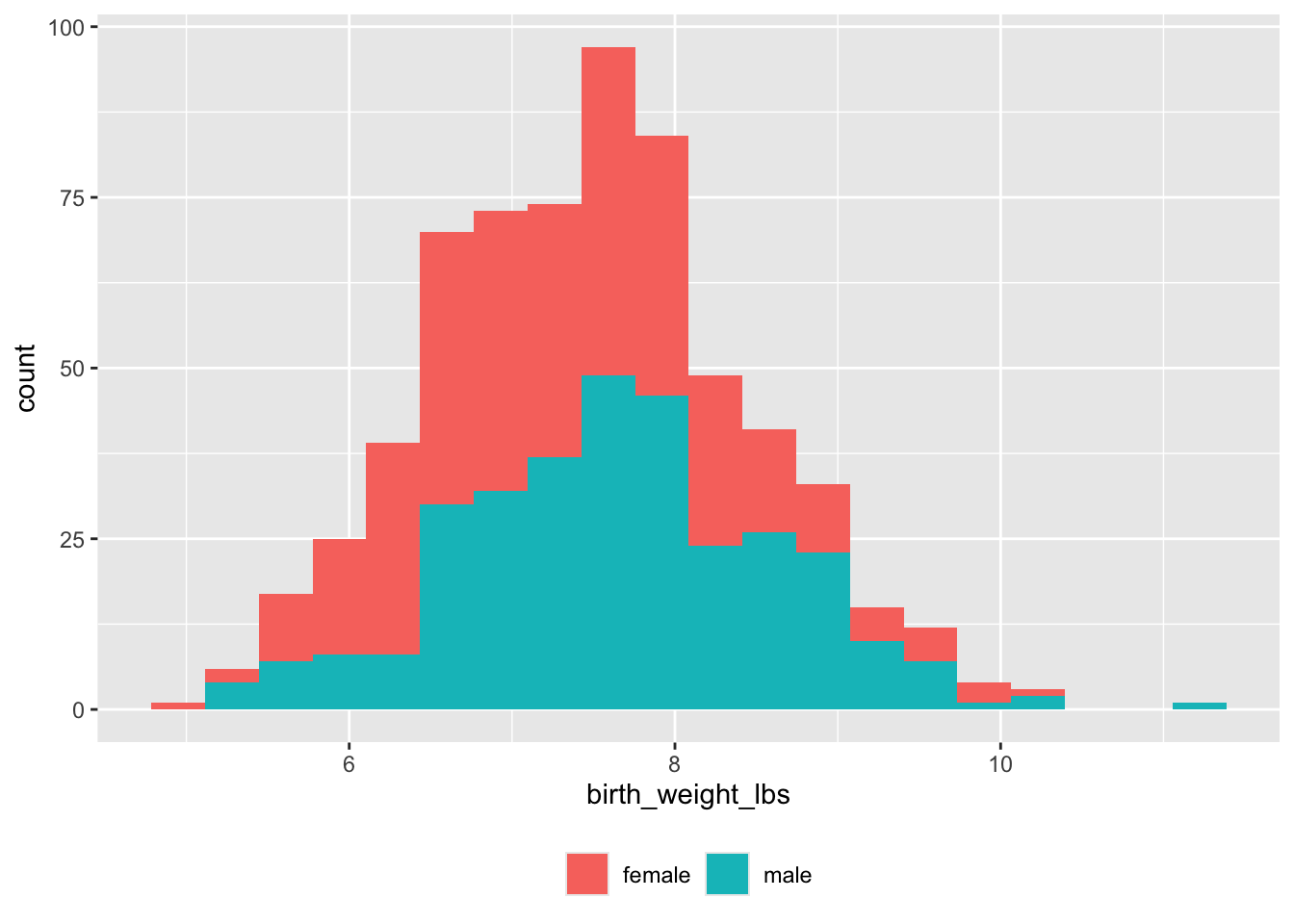
Birth complications
xtabs(formula = ~ child_sex + child_birth_complications,
      data = screen_df)
## child_birth_complications
## child_sex no yes
## female 290 30
## male 282 24There are some first names in the child_birth_complications_specify field, so it is not shown here.
Major illnesses or injuries
xtabs(formula = ~ child_sex + child_major_illnesses_injuries,
      data = screen_df)
## child_major_illnesses_injuries
## child_sex no yes
## female 308 12
## male 294 12
screen_df |>
  dplyr::filter(!is.na(child_illnesses_injuries_specify),
                !stringr::str_detect(child_illnesses_injuries_specify, "OK")) |>
  dplyr::select(child_age_mos, child_sex, child_illnesses_injuries_specify) |>
  dplyr::arrange(child_age_mos) |>
knitr::kable(format = 'html')| child_age_mos | child_sex | child_illnesses_injuries_specify |
|---|---|---|
| 11.40697 | female | COVID in January, no later complications. |
| 11.86719 | female | RSV when she 3 months; was in hospital for 2 nights |
| 12.68902 | female | fractured wrist when she was 9 months |
| 12.73285 | male | He had Covid once. |
| 12.76162 | female | RSV when 10 weeks old, hospitalized for 1 week |
| 13.01775 | male | Covid in December but this did NOT result in a visual, auditory, motor, or cognitive disability according to mom |
| 13.02186 | male | Respiratory failure and sepsis after birth that was resolved |
| 16.17494 | female | Child had a fall but she was fine. |
| 17.81860 | female | **bit by tick a couple months ago, took meds to prevent Lyme disease |
| 18.04597 | female | broke leg in April - all healed now. slide accident, she was 16 months. in a cast for three weeks, and then a week phantom limping. |
| 18.18020 | female | Respiratory Syncytial Virus(RSV) |
| 18.67330 | male | tibial stress factor |
| 18.70617 | male | RSV but did not need to be admitted. This illness did not result in an impairment or disability. |
| 18.77055 | male | Child had COVID twice (fever, etc.) |
| 20.67856 | male | Anaphylactic reaction to peanuts |
| 22.48658 | female | Child was born with a heart murmur- cardiologist said she is unaffected and will likely grow out of it. Child also had an isolated febrile seizure short after 1st birthday. Has not experienced a seizure since. |
| 23.01118 | male | He had RSV then COVID around 13-14 months old, but they were both very mild. No complications arose from either. |
| 23.20979 | female | febrile seizure- around 1 1/2 years |
| 24.03024 | male | had COVID at 7 months |
| 24.91782 | female | She had COVID, and when she was little had an cardiac issue (her heart was "working" too hard) but she was okay soon after (this was first 2-3 months after birth). March of 2021 she had fully recovered from this, and received treatment |
| 25.70814 | male | hospital day 4 for hypothermia - then negative / no diagnosis |
| 26.76008 | male | Has had a fall, was a concussion but not diagnosed with any disabilities |
| 32.67724 | male | Pneumonia at 5 months |
Child vision
xtabs(formula = ~ child_sex + child_vision_disabilities,
      data = screen_df)
## child_vision_disabilities
## child_sex no yes
## female 318 2
## male 304 2
screen_df |>
  dplyr::filter(!is.na(child_vision_disabilities_specify)) |>
  dplyr::select(child_age_mos, child_sex, child_vision_disabilities_specify) |>
  dplyr::arrange(child_age_mos) |>
knitr::kable(format = 'html')| child_age_mos | child_sex | child_vision_disabilities_specify |
|---|---|---|
| 18.70617 | male | He wears glasses to correct his far sighted vision. He does not have vision loss. |
| 22.35371 | female | She has a lazy eye, she wears an eye patch for part of the day. |
| 23.14267 | female | Strabismus - wears glasses |
| 24.03024 | male | lazy eye but corrected |
Child hearing
xtabs(formula = ~ child_sex + child_hearing_disabilities,
      data = screen_df)
## child_hearing_disabilities
## child_sex no yes
## female 320 0
## male 305 1
screen_df |>
  dplyr::filter(!is.na(child_hearing_disabilities_specify)) |>
  dplyr::select(child_age_mos, child_sex, child_hearing_disabilities_specify) |>
  dplyr::arrange(child_age_mos) |>
knitr::kable(format = 'html')| child_age_mos | child_sex | child_hearing_disabilities_specify |
|---|---|---|
| 32.67724 | male | Temporary hearing loss so tubes in his ears, one still remaining |
Child developmental delays
xtabs(formula = ~ child_sex + child_developmentaldelays,
      data = screen_df)
## child_developmentaldelays
## child_sex no yes
## female 254 3
## male 246 5There may be first names in the child_developmentaldelays_specify field, so it is not shown here.
Child sleep
This is work yet-to-be-done. The time stamps need to be reformatted prior to visualization.
Bed time
extract_sleep_hr <- function(t) {
  t |>
    stringr::str_extract("^[0-9]{2}\\:[0-9]{2}\\:[0-9]{2}") |>
    hms::as_hms()
}

df <- screen_df |>
  dplyr::mutate(child_sleep_time = extract_sleep_hr(child_sleep_time)) |>
  dplyr::filter(!is.na(child_sleep_time))

df |>
  dplyr::filter(!is.na(child_sleep_time),
                !is.na(child_sex)) |>
  ggplot() +
  aes(child_sleep_time, fill = child_sex) +
  geom_histogram(bins = 18) +
  theme(legend.position = "bottom") +
  theme(legend.title = element_blank())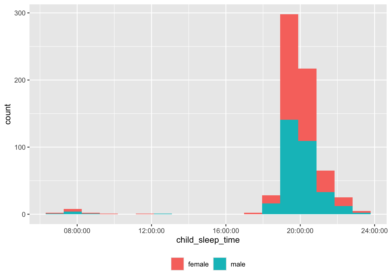
Some of the bed times are probably not in correct 24 hr time.
df |>
  dplyr::filter(child_sleep_time < hms::as_hms("16:00:00")) |>
  dplyr::select(site_id, participant_ID, child_sleep_time) |>
  dplyr::arrange(site_id, participant_ID) |>
knitr::kable('html')| site_id | participant_ID | child_sleep_time |
|---|---|---|
| CSUFL | 013 | 07:00:00 |
| CSULB | 006 | 07:30:00 |
| INDNA | 004 | 09:00:00 |
| INDNA | 006 | 07:45:00 |
| NYUNI | 082 | 07:00:00 |
| OHIOS | 002 | 10:00:00 |
| PRINU | 001 | 12:15:00 |
| PRINU | 018 | 07:30:00 |
| PRINU | 027 | 07:30:00 |
| PURDU | 020 | 08:30:00 |
| PURDU | 021 | 11:30:00 |
| UCSCR | 011 | 07:30:00 |
| UGEOR | 016 | 07:30:00 |
| UTAUS | 023 | 08:00:00 |
Wake time
df <- screen_df |>
  dplyr::mutate(child_wake_time = extract_sleep_hr(child_wake_time)) |>
  dplyr::filter(!is.na(child_wake_time))

df |>
  dplyr::filter(!is.na(child_wake_time),
                !is.na(child_sex)) |>
  ggplot() +
  aes(child_wake_time, fill = child_sex) +
  geom_histogram(bins = 18) +
  theme(legend.position = "bottom") +
  theme(legend.title = element_blank())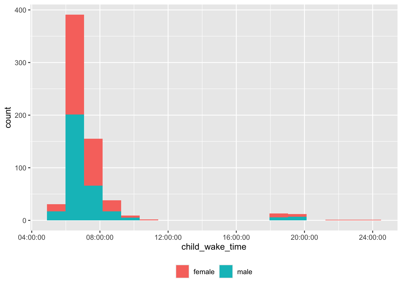
There are some unusual wake times, too.
df |>
  dplyr::filter(child_wake_time > hms::as_hms("16:00:00")) |>
  dplyr::select(site_id, participant_ID, child_wake_time) |>
  dplyr::arrange(site_id, participant_ID) |>
knitr::kable('html')| site_id | participant_ID | child_wake_time |
|---|---|---|
| BOSTU | 001 | 19:30:00 |
| CHOPH | 017 | 19:30:00 |
| GEORG | 026 | 19:00:00 |
| OHIOS | 009 | 18:30:00 |
| OHIOS | 012 | 19:30:00 |
| OHIOS | 014 | 18:30:00 |
| OHIOS | 018 | 18:45:00 |
| OHIOS | 019 | 19:30:00 |
| OHIOS | 021 | 19:30:00 |
| OHIOS | 029 | 19:30:00 |
| OHIOS | 031 | 19:30:00 |
| OHIOS | 035 | 19:00:00 |
| OHIOS | 062 | 18:30:00 |
| PRINU | 015 | 19:00:00 |
| PRINU | 018 | 19:45:00 |
| PRINU | 027 | 20:00:00 |
| PURDU | 020 | 21:30:00 |
| PURDU | 021 | 23:30:00 |
| PURDU | 023 | 23:00:00 |
| UCRIV | 007 | 18:00:00 |
| UCSCR | 035 | 18:30:00 |
| UGEOR | 002 | 19:30:00 |
| UHOUS | 014 | 19:00:00 |
| UMIAM | 013 | 20:00:00 |
| UTAUS | 013 | 18:00:00 |
| UTAUS | 020 | 18:30:00 |
| UTAUS | 040 | 19:00:00 |
| UTAUS | 043 | 19:15:00 |
Sleep duration
df <- screen_df |>
  dplyr::mutate(child_sleep_time = extract_sleep_hr(child_sleep_time),
                  child_wake_time = extract_sleep_hr(child_wake_time)) |>
  dplyr::filter(!is.na(child_sleep_time),
                !is.na(child_wake_time)) |>
  dplyr::mutate(child_sleep_secs = (child_sleep_time - child_wake_time))

df |>
  dplyr::filter(!is.na(child_sleep_secs)) |>
  ggplot() +
  aes(child_sleep_secs, fill = child_sex) +
  geom_histogram(bins = 18) +
  theme(legend.position = "bottom") +
  theme(legend.title = element_blank())
## Don't know how to automatically pick scale for object of type <difftime>.
## Defaulting to continuous.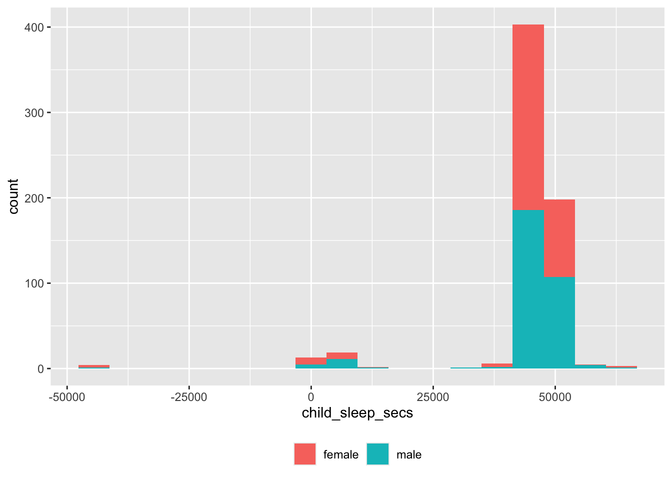
Again, there are some unusual values.
df |>
  dplyr::filter(child_sleep_secs < 12000) |>
  dplyr::select(site_id, participant_ID, child_sleep_time, child_wake_time, child_sleep_secs) |>
  dplyr::arrange(site_id, participant_ID) |>
knitr::kable('html')| site_id | participant_ID | child_sleep_time | child_wake_time | child_sleep_secs |
|---|---|---|---|---|
| BOSTU | 001 | 19:30:00 | 19:30:00 | 0 secs |
| CHOPH | 017 | 20:45:00 | 19:30:00 | 4500 secs |
| CSUFL | 013 | 07:00:00 | 06:00:00 | 3600 secs |
| CSULB | 006 | 07:30:00 | 07:30:00 | 0 secs |
| GEORG | 026 | 19:45:00 | 19:00:00 | 2700 secs |
| INDNA | 004 | 09:00:00 | 08:00:00 | 3600 secs |
| INDNA | 006 | 07:45:00 | 06:30:00 | 4500 secs |
| NYUNI | 082 | 07:00:00 | 06:15:00 | 2700 secs |
| OHIOS | 002 | 10:00:00 | 08:00:00 | 7200 secs |
| OHIOS | 009 | 18:30:00 | 18:30:00 | 0 secs |
| OHIOS | 012 | 20:00:00 | 19:30:00 | 1800 secs |
| OHIOS | 014 | 20:00:00 | 18:30:00 | 5400 secs |
| OHIOS | 018 | 20:00:00 | 18:45:00 | 4500 secs |
| OHIOS | 019 | 20:30:00 | 19:30:00 | 3600 secs |
| OHIOS | 021 | 20:00:00 | 19:30:00 | 1800 secs |
| OHIOS | 029 | 20:45:00 | 19:30:00 | 4500 secs |
| OHIOS | 031 | 20:30:00 | 19:30:00 | 3600 secs |
| OHIOS | 035 | 20:30:00 | 19:00:00 | 5400 secs |
| OHIOS | 062 | 20:30:00 | 18:30:00 | 7200 secs |
| PRINU | 015 | 19:00:00 | 19:00:00 | 0 secs |
| PRINU | 018 | 07:30:00 | 19:45:00 | -44100 secs |
| PRINU | 027 | 07:30:00 | 20:00:00 | -45000 secs |
| PURDU | 020 | 08:30:00 | 21:30:00 | -46800 secs |
| PURDU | 021 | 11:30:00 | 23:30:00 | -43200 secs |
| PURDU | 023 | 22:30:00 | 23:00:00 | -1800 secs |
| UCRIV | 007 | 21:00:00 | 18:00:00 | 10800 secs |
| UCSCR | 011 | 07:30:00 | 06:30:00 | 3600 secs |
| UCSCR | 035 | 20:45:00 | 18:30:00 | 8100 secs |
| UGEOR | 002 | 20:00:00 | 19:30:00 | 1800 secs |
| UGEOR | 016 | 07:30:00 | 08:00:00 | -1800 secs |
| UHOUS | 014 | 19:00:00 | 19:00:00 | 0 secs |
| UMIAM | 013 | 21:00:00 | 20:00:00 | 3600 secs |
| UTAUS | 013 | 19:30:00 | 18:00:00 | 5400 secs |
| UTAUS | 020 | 20:00:00 | 18:30:00 | 5400 secs |
| UTAUS | 023 | 08:00:00 | 07:00:00 | 3600 secs |
| UTAUS | 040 | 19:00:00 | 19:00:00 | 0 secs |
| UTAUS | 043 | 22:00:00 | 19:15:00 | 9900 secs |
Nap hours
df <- screen_df |>
  dplyr::mutate(child_nap_hours = as.numeric(child_nap_hours)) |>
  dplyr::filter(!is.na(child_sleep_time))
## Warning: There was 1 warning in `dplyr::mutate()`.
## ℹ In argument: `child_nap_hours = as.numeric(child_nap_hours)`.
## Caused by warning:
## ! NAs introduced by coercion
df |>
  dplyr::filter(!is.na(child_nap_hours),
                !is.na(child_sex)) |>
  ggplot() +
  aes(child_nap_hours, fill = child_sex) +
  geom_histogram(bins = 18) +
  theme(legend.position = "bottom") +
  theme(legend.title = element_blank())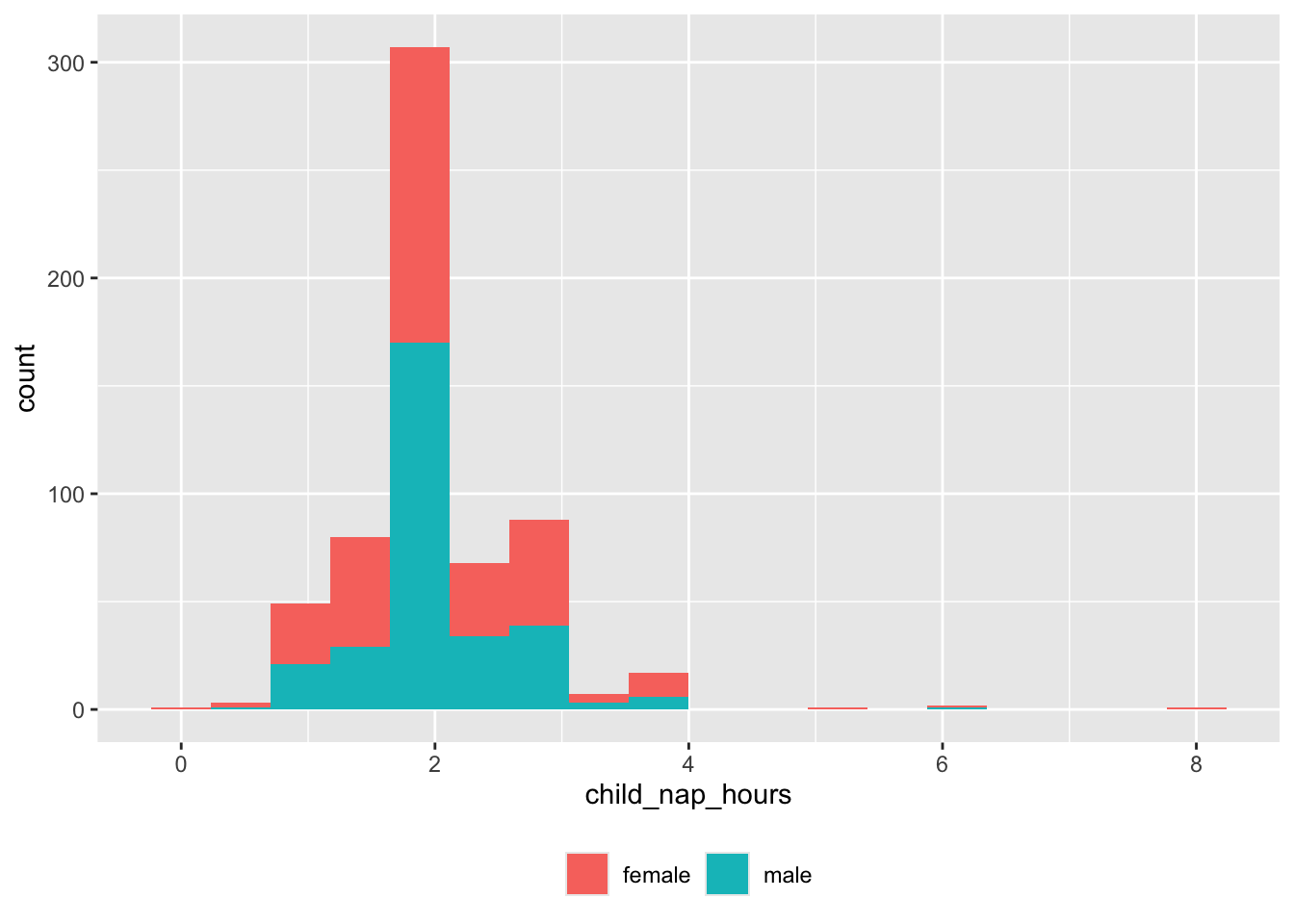
And there are some very long nappers or null values we need to capture.
df |>
  dplyr::filter(child_nap_hours > 5) |>
  dplyr::select(site_id, participant_ID, child_nap_hours) |>
  dplyr::arrange(site_id, participant_ID) |>
knitr::kable('html')| site_id | participant_ID | child_nap_hours |
|---|---|---|
| UMIAM | 003 | 8 |
| UTAUS | 009 | 6 |
Sleep location
xtabs(formula = ~ child_sex + child_sleep_location,
      data = screen_df)
Mother
Biological or adoptive
xtabs(formula = ~ child_sex + mom_bio,
      data = screen_df)
## mom_bio
## child_sex no_partnerchild yes
## female 1 305
## male 0 301Age at childbirth
screen_df |>
  dplyr::filter(!is.na(mom_childbirth_age), !is.na(child_sex)) |>
  ggplot() +
  aes(x = mom_childbirth_age, fill = child_sex) +
  geom_histogram(bins = 25) +
  theme(legend.position = "bottom") +
  theme(legend.title = element_blank())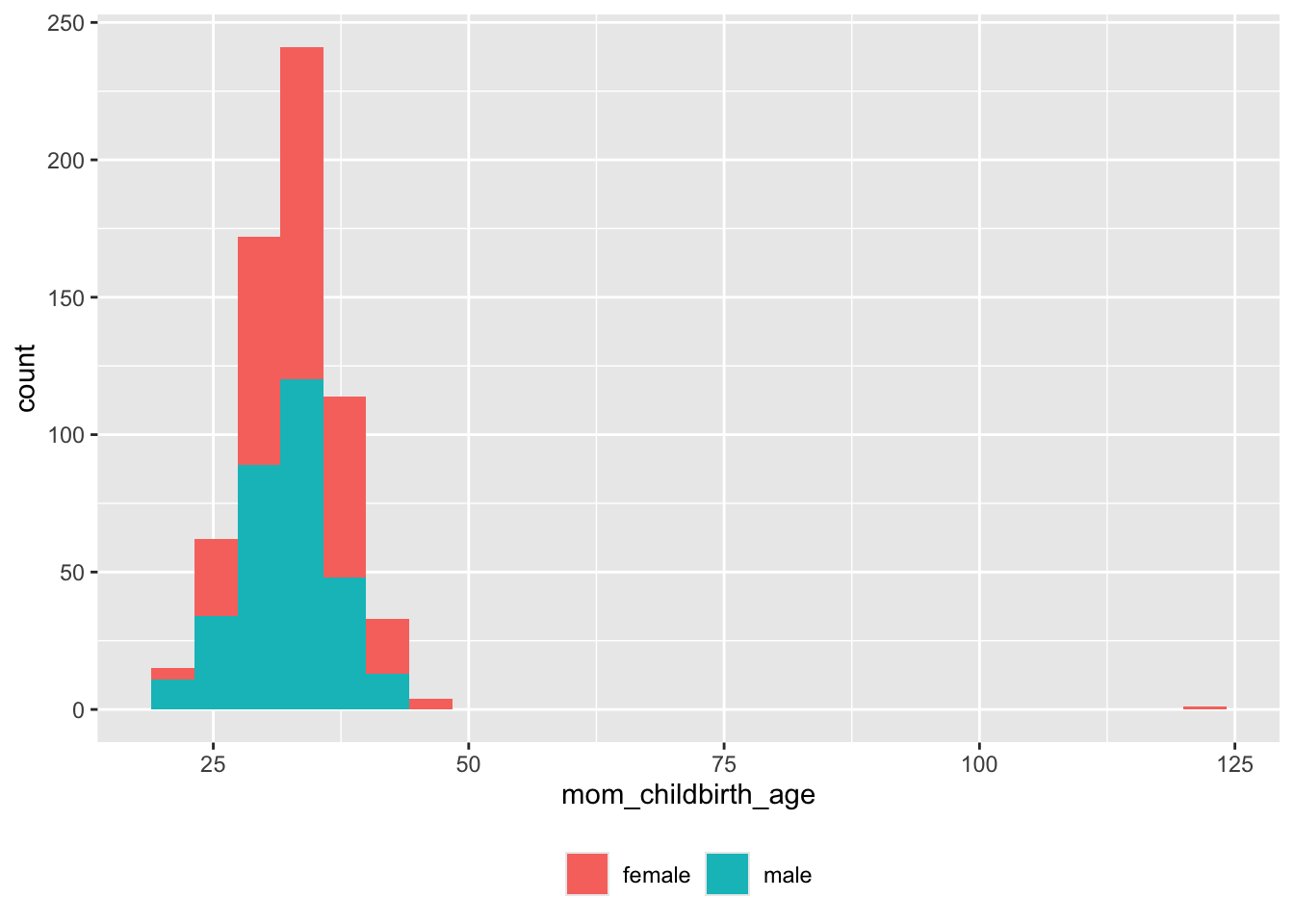
Clearly, there are some impossible (erroneous) maternal ages > 100. Here are details:
old_moms <- screen_df |>
  dplyr::filter(mom_childbirth_age > 55)

old_moms |>
  dplyr::select(submit_date, vol_id, participant_ID, mom_childbirth_age) |>
knitr::kable(format = 'html')| submit_date | vol_id | participant_ID | mom_childbirth_age |
|---|---|---|---|
| 2022-07-07 15:03:20 | 1391 | 005 | 121.22 |
Race
df <- screen_df |>
  dplyr::filter(!is.na(mom_race)) |>
  dplyr::mutate(mom_race = dplyr::recode(
    mom_race,
    morethanone = "more_than_one",
    americanindian = "american_indian"))

xtabs(~mom_race, df)
## mom_race
## american_indian asian black more_than_one
## 2 19 24 33
## other refused white
## 38 2 502Birth country
df <- screen_df |>
  dplyr::mutate(mom_birth_country = dplyr::recode(
    mom_birth_country,
    unitedstates = "US",
    united_states = "US",
    othercountry = "Other",
    other_country = "Other",
    refused = "Refused"
  ))

xtabs(~ mom_birth_country, data = df)
## mom_birth_country
## Other puertorico US
## 76 3 541
df <- screen_df |>
  dplyr::mutate(mom_birth_country_specify = stringr::str_to_title(mom_birth_country_specify)) |>
  dplyr::filter(!is.na(mom_birth_country_specify)) |>
  dplyr::select(child_sex, mom_birth_country_specify)

unique(df$mom_birth_country_specify)
## [1] "South Korea" "Argentina" "Spain"
## [4] "Zimbabwe" "Mexico" "Bolivia"
## [7] "Canada" "Uk" "Refused"
## [10] "United Kingdom" "Australia" "Venezuela"
## [13] "India" "Kenya" "England"
## [16] "China" "Ireland" "El Salvador"
## [19] "Colombia" "Chile" "Guatemala"
## [22] "Ecuador" "Costa Rica" "Italy"
## [25] "Malaysia" "Phillipines" "Dominican Republic"
## [28] "Nigeria" "Honduras" "Colomobia"
## [31] "Columbia" "Panama"Education
df <- screen_df |>
  dplyr::filter(!is.na(mom_education)) |>
  dplyr::select(child_sex, mom_education)

xtabs(~ mom_education, data = df)
## mom_education
## associates bachelor_s_deg bachelors diploma
## 18 3 203 18
## doctorate ged graduate_nodegree master_s_degre
## 80 3 17 2
## masters ninth professional professional_d
## 208 1 32 2
## somecollege voc_diplima voc_nodiplima
## 30 1 1This requires some recoding work.
Occupation
This information is available, but would need to be substantially recoded to be useful in summary form.
Jobs number
## mom_jobs_number
##   0   1   2   3   4
##   1 428  51   1   1
df <- screen_df |>
  dplyr::filter(!is.na(mom_jobs_number),
                !is.na(mom_employment))

xtabs(~ mom_jobs_number + mom_employment, data = df)
## mom_employment
## mom_jobs_number full_time part_time
## 0 0 1
## 1 335 93
## 2 29 22
## 3 1 0
## 4 1 0Biological father
Race
df <- screen_df |>
  dplyr::select(biodad_childbirth_age, biodad_race, child_sex) |>
  dplyr::mutate(
    biodad_race =
      dplyr::recode(
        biodad_race,
        americanindian_NA = "american_indian",
        asian_NA = "asian",
        NA_asian = "asian",
        black_NA = "black",
        donotknow_NA = "do_not_know",
        NA_NA = "NA",
        NA_white = "white",
        other_NA = "other",
        refused_NA = "refused",
        white_NA = "white",
        morethanone_NA = "more_than_one"
      )
  ) |>
  dplyr::mutate(biodad_childbirth_age = stringr::str_remove_all(biodad_childbirth_age, "[_NA]")) |>
  # dplyr::filter(!is.na(biodad_childbirth_age), !is.na(biodad_race)) |>
  dplyr::mutate(biodad_childbirth_age = as.numeric(biodad_childbirth_age))
## Warning: There was 1 warning in `dplyr::mutate()`.
## ℹ In argument: `biodad_childbirth_age =
## as.numeric(biodad_childbirth_age)`.
## Caused by warning:
## ! NAs introduced by coercion
xtabs(~ biodad_race, df)## biodad_race
## american_indian asian black do_not_know
## 3 21 29 3
## more_than_one NA nativehawaiian_NA other
## 24 29 1 52
## refused white
## 3 471Age at child birth
df |>
  dplyr::filter(!is.na(biodad_childbirth_age)) |>
  ggplot() +
  aes(x = biodad_childbirth_age, fill = child_sex) +
  geom_histogram(bins = 25) +
  theme(legend.position = "bottom") +
  theme(legend.title = element_blank())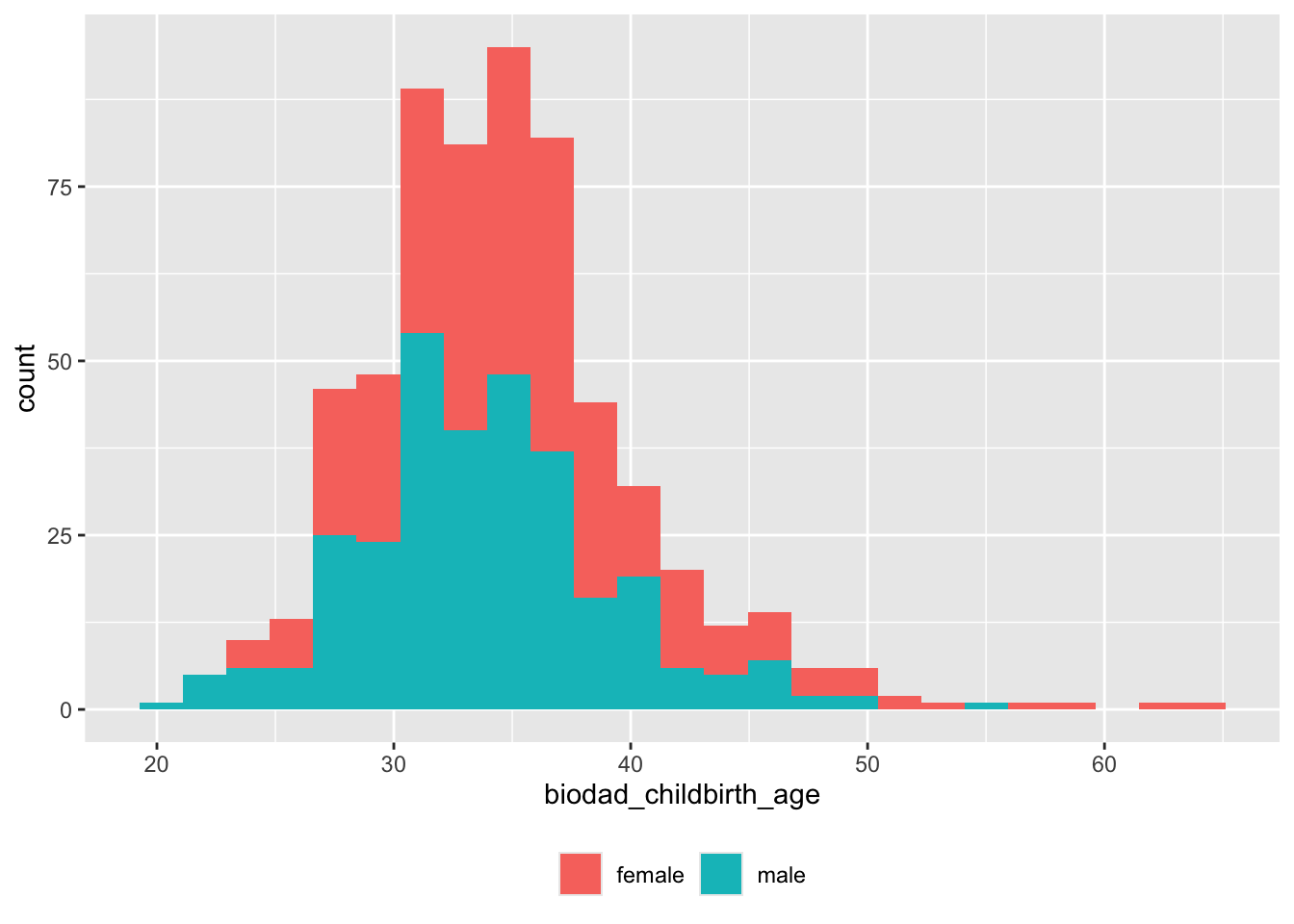
Childcare
Types
## childcare_types
##                childcare           childcare_cent
##                      167                        2
##                    nanny           nanny_babysitt
##                        4                        1
##               nanny_home     nanny_home childcare
##                       29                       10
## nanny_home nanny_nothome      nanny_home relative
##                        2                        5
##            nanny_nothome  nanny_nothome childcare
##                       11                        3
##   nanny_nothome relative                     none
##                        1                      118
##                 relative       relative childcare
##                       66                       13
This requires some cleaning.
Hours
df <- screen_df |>
  dplyr::filter(!is.na(childcare_hours)) |>
  dplyr::arrange(childcare_hours)

unique(df$childcare_hours)
## [1] "1"
## [2] "10"
## [3] "12"
## [4] "13"
## [5] "14"
## [6] "14.5"
## [7] "15"
## [8] "15-20"
## [9] "16"
## [10] "16-20"
## [11] "17.5"
## [12] "18"
## [13] "2"
## [14] "2-3"
## [15] "2-4"
## [16] "20"
## [17] "20 hours"
## [18] "20 hours a week - maternal grandmother"
## [19] "21"
## [20] "21 (14 hr childcare center, 7 hr babysitter)"
## [21] "24"
## [22] "25"
## [23] "25, 15 of those hours are at daycare"
## [24] "26"
## [25] "27"
## [26] "28"
## [27] "3"
## [28] "30"
## [29] "30-35"
## [30] "30-40"
## [31] "31"
## [32] "32"
## [33] "33"
## [34] "34"
## [35] "35"
## [36] "35-40"
## [37] "36"
## [38] "36; Grandpa watches one day a week"
## [39] "37"
## [40] "38"
## [41] "4"
## [42] "40"
## [43] "40+"
## [44] "40-45"
## [45] "40-50"
## [46] "42"
## [47] "42.5"
## [48] "43"
## [49] "45"
## [50] "45-50"
## [51] "47"
## [52] "5"
## [53] "50"
## [54] "52.5"
## [55] "53"
## [56] "6"
## [57] "63"
## [58] "8"
## [59] "8-16"
## [60] "8-5 each day"
## [61] "80"
## [62] "9"This requires some cleaning.
Language
##  [1] "Spanish and English (half and half)"
##  [2] "English"
##  [3] "Spanish"
##  [4] "English and Spanish (50/50)"
##  [5] "english"
##  [6] "English when speaking with children, but Arabic when speaking to eachother"
##  [7] "Mostly English, some Spanish"
##  [8] "Mandarin"
##  [9] "Spanish at the center"
## [10] "English and Spanish"
## [11] "English, Spanish"
## [12] "Usually English, sometimes arabic and french"
## [13] "English and speaks a little bit of Japanese but not directly to Lucas"
## [14] "English and Creole"
## [15] "Spanish (sometimes English)"
## [16] "English;Spanish"
## [17] "Spanish and English"
## [18] "spanish"
## [19] "French only"
## [20] "English and some sign language"
## [21] "English, American Sign Language"
## [22] "English and ASL"
## [23] "Ingles"
## [24] "English/Spanish"
## [25] "English and some Spanish"
## [26] "Nanny in Spanish at home. At school both English and Spanish."
## [27] "English (majority of the time) and sometimes Spanish"
## [28] "English and Spanish 50/50"
## [29] "english, some spanish"
## [30] "English, sometimes a little bit of Spanish"
## [31] "English &  Spanish"
This requires some cleaning.